OXASL walk through tutorial - GUI
This tutorial demonstrates some of the common options available in the OXASL GUI.
We will be working with single and multi-PLD data from the FSL tutorial on Arterial Spin Labelling. You will need to download the data from this link before following the tutorial.
The tutorial has been written so that we start with the most basic analysis and gradually add options and show the effect they have on the output, as well as how they are reported in the command log and the summary report. However this is not a complete description of all available options in the GUI or the command line - for that see the OXASL walk through tutorial - command line or OXASL command reference.
Perfusion quantification using Single PLD pcASL
The aim of this exercise is to perform perfusion quantification with one of the most widely recommened variants of ASL. Single PLD pcASL is now regarded as sufficiently simple and reliable, both for acquisition and analysis, that it is the first option most people should consider when using ASL for the first time. Although more can be done with other ASL variants, particularly when acquisition time allows.
The data
This dataset used pcASL labeling and we are going to start with data collected using a single post-label delay. This dataset follows as closely as possible the recommendations of the ASL Consensus Paper (commonly called the ‘White Paper’) on a good general purpose ASL acquisition, although we have chosen to use a 2D mutli-slice readout rather than a full-volume 3D readout.
The files you will need to begin with are:
spld_asltc.nii.gz- the label-control ASL series containing 60 volumes. That is 30 label and 30 control, in pairs of alternating images with label first.
aslcalib.nii.gz- the calibration image, a (largely) proton-density weighted image with the same readout (resolution etc) as the main ASL data. The TR for this data is 4.8 seconds, which means there will be some T1 weighting.
aslcalib_PA.nii.gz- another calibration image, identical toaslcalib.nii.gzapart from the use of posterior-anterior phase encoding (anterior-posterior was used in the rest of the ASL data). This is provided for distortion correction.
T1.nii.gz- the T1-weigthed anatomical of the same subject.
To launch the GUI at the command line you will need to type
oxasl_gui. Note that if you have downloaded the
‘pre-release’ yourself, you may need to provide a path to the
installed version of the GUI, e.g. /Users/{blah}/Downloads/oxasl/oxasl_gui
Once it has launched you will find yourself on the ‘Input Data’ tab, you should:
Load the ASL data
spld_asltc.nii.gzas the ‘Input Image’.Set the ‘Number of PLDs’, which in this case is 1, this is already done by default.
Click the ‘Update’ button beneath the ‘Data Preview’ pane on the right.
At this point the GUI should look like the screen shot below and a perfusion weighted image will have appeared in the ‘Data Preview’ pane. This this is reassuring, if we didn’t see something that looks roughly like this, we might check if the data order that the GUI is expecting matches that in the data. We could alter the ‘Data order’ settings if needed and update the preview again.
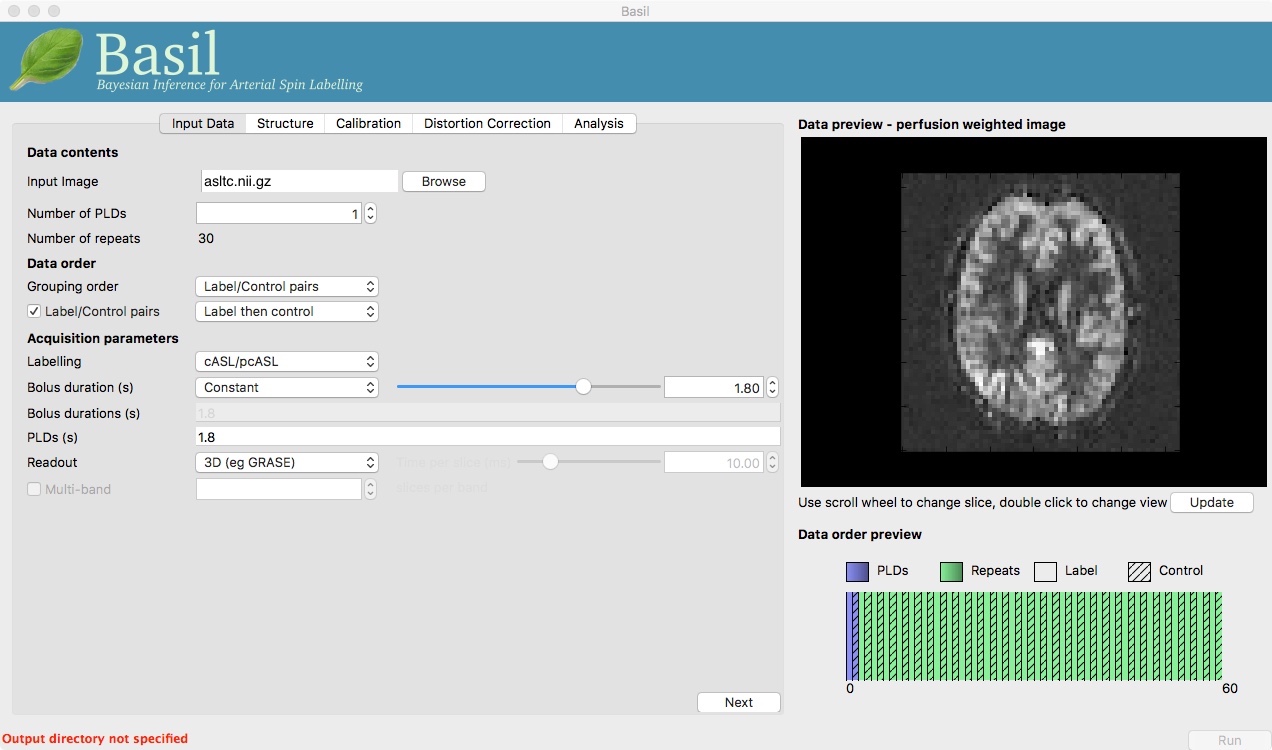
Note also, beneath the ‘Data Preview’, that there is a ‘Data order preview’. The idea of this graphic is to help visually to confirm that the way that the GUI is intepreting the ordering of volumes in the data matches what you are expecting. In this case we have a single PLD repeated 30 times with the label and control images paired in the data (this is pretty common). What the ‘Data order preview’ shows is the first instance of the PLD in purple, showing both the label and control (hatched) volume. Each subsequent repeat of the same PLD is coloured green, again showing that we have a label follwed by control (hatched) volume.
You can try a different ‘Data order’ option to see what happens. Change ‘Label/Control pairs’ from ‘Label then control’ to ‘Control then label’. This switches the expected order of label and control images within the pair. If you then udpate the preview you will find that the contrast reverses, the perfusion now has the wrong ‘sign’.
(Simple) Perfusion Quantification
We have checked the PWI, thus we can proceed to final quantification of perfusion, inverting the kinetics of the ASL label delivery and using the calibration image to get values in the units of ml/100g/min.
To do this we need to tell the BASIL GUI some information about the data and the analysis we want to perform.
On the ‘Input Data’ tab we need to sepcify the ‘Acquisition parameters’:
Labelling - cASL/pcASL (the deafult option).
Bolus duration (s) - 1.8 (default).
PLDs (s) - 1.8 (default).
Readout - 2D multi-slice (you will need to set this).
Time per slice (ms) - 45.2 (only appears when you change the Readout option).
You can now hit ‘Next’ and you will be taken to the next tab. For this (simple) analysis we do not want to use a structural image, so we can move on by clicking ‘Next’ again. Or we could skip stright to the ‘Calibration’ tab using the menu across the top.
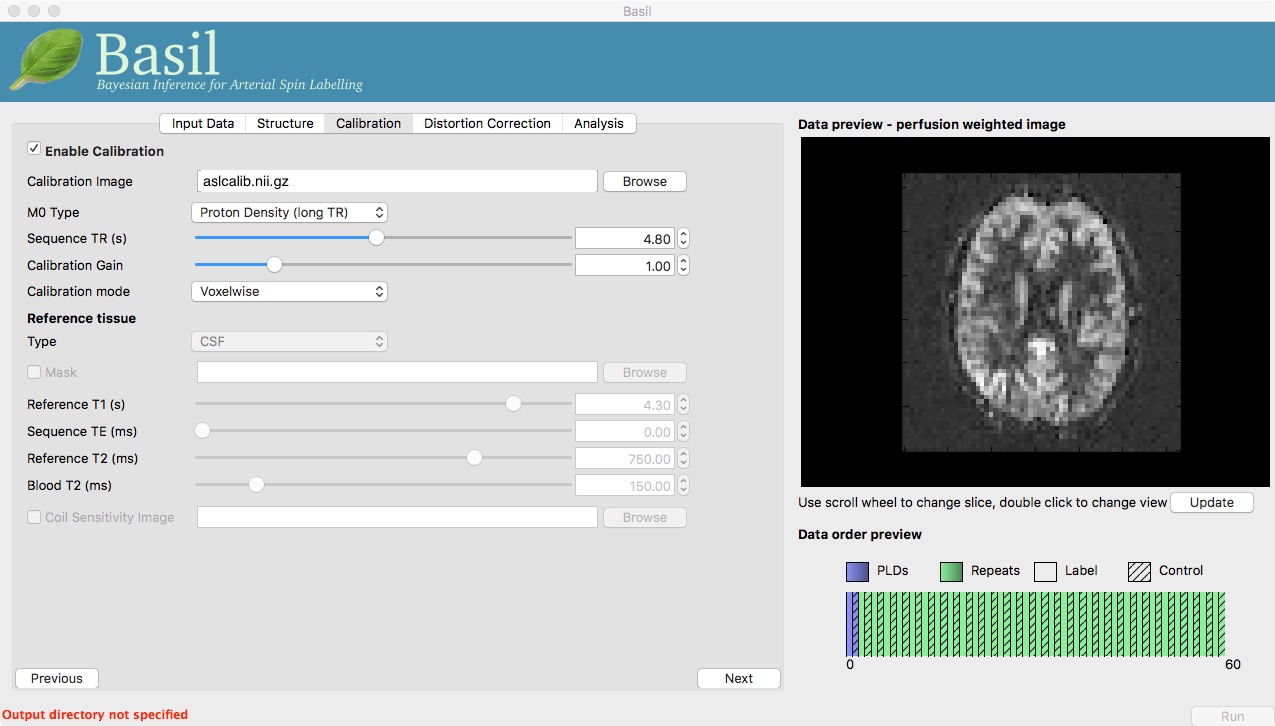
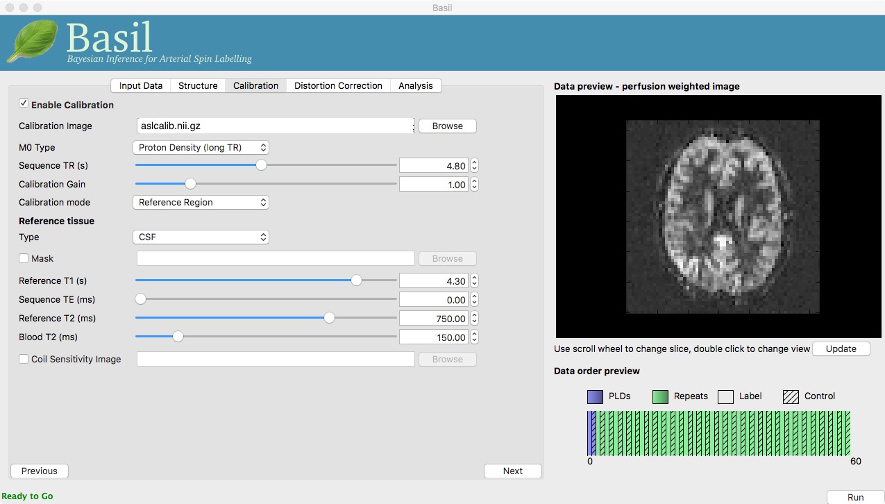
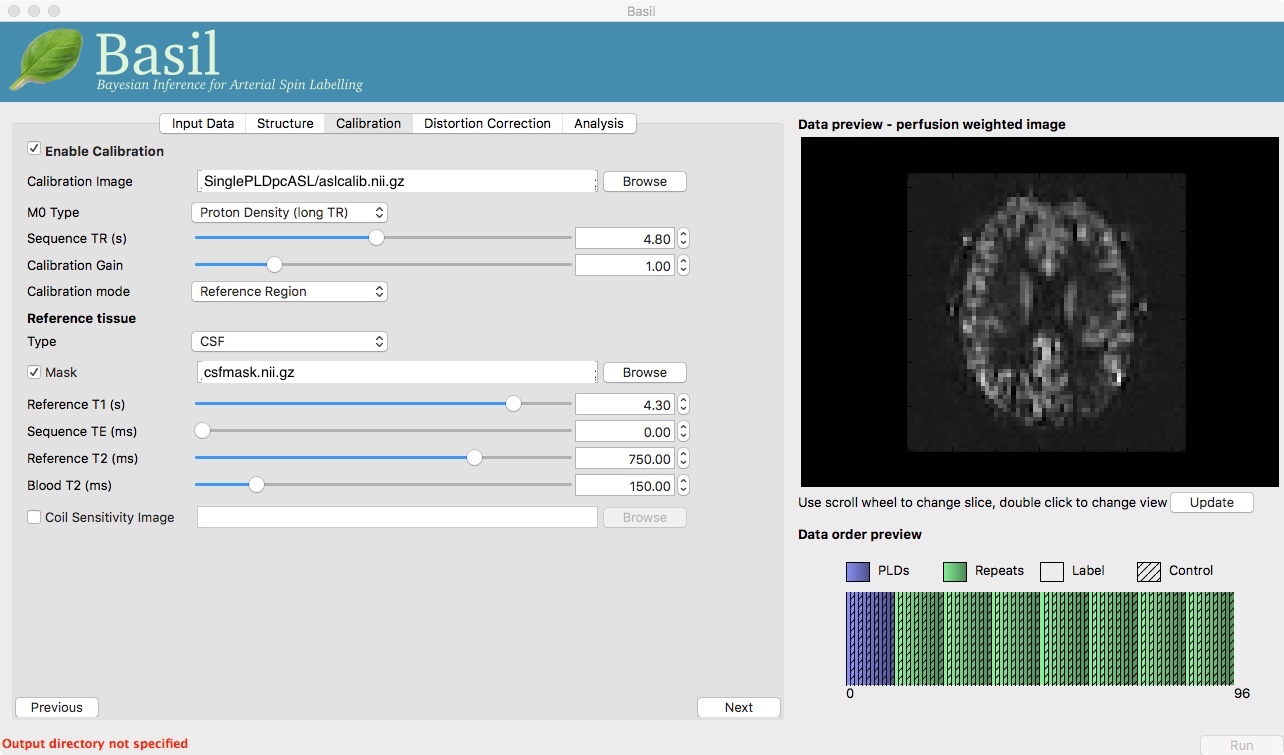
On the ‘Calibration’ tab, ‘Enable Calibration’ first, then load
the calibration image aslcalib.nii.gz. Change the
‘Calibration mode’ to ‘voxelwise’, and set the ‘Sequence TR (s)’ to
be 4.8.
Finally, we need to set the analysis options: either skip to the ‘Analysis’ tab or click ‘Next’ twice.
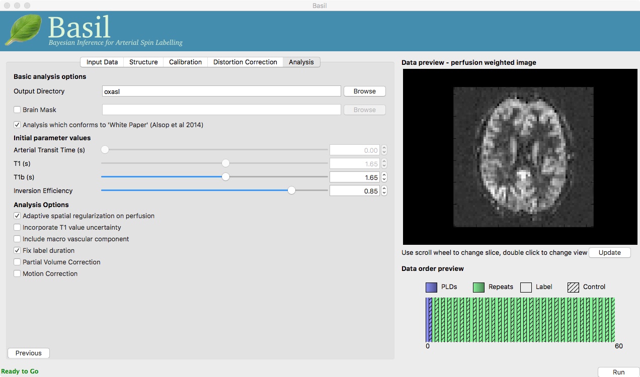
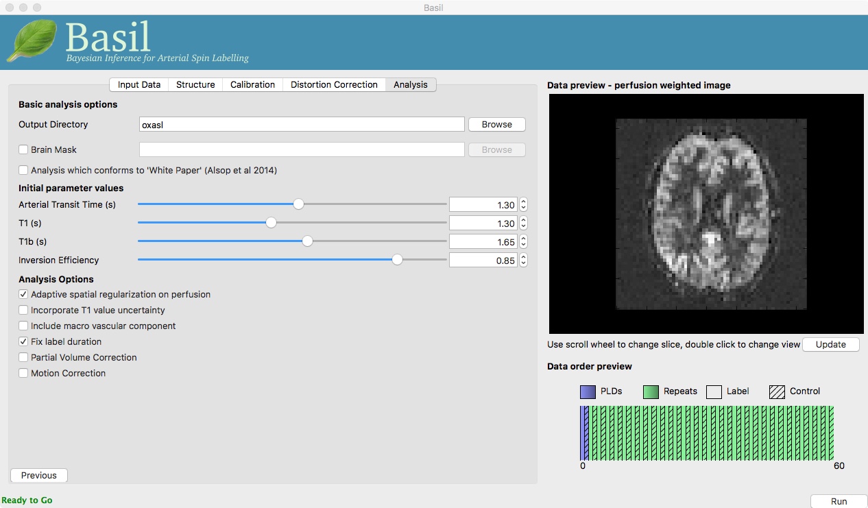
On the ‘Analysis’ tab, choose an output directory name, e.g.,
oxasl. And, select ‘Analysis which conforms to White
Paper’, so that we know the analysis is using the same default
parameter values proposed in the ‘ASL White Paper’ quantification
formula. Note that in the lower left corner the GUI is now telling
us that we are ‘Ready to Go’. At this point you can click ‘Run’ in
the lower right corner.
The output of the oxasl command line tool is shown in a
pop-up window. You can ignore any erfc underflow error messages
- they are harmless and occur because we haven’t provided any
structural data
This analysis should only take a few minutes, but while you are waiting you can read ahead and even start changing the options in the GUI ready for the next analysis that we want to run.
Once the analysis had completed, view the final result:
fsleyes oxasl/output/native/calib_voxelwise/perfusion.nii.gz
Note that if you just supply a name for the output directory (not a full path), as we have here, this will be placed in the ‘working directory’, i.e. whichever directory you were in when you launched the GUI.
You will find something that looks very similar to the PWI we viewed before, but now the values at every voxel are in ml/100g/min.
You will also find a PWI saved as
oxasl/output/native/perfusion. This is very similar to the
PWI displayed in the preview pane, except that the kinetic
model inversion has been applied to it, this is the image
pre-calibration.
Improving the Perfusion Images from single PLD pcASL
The purpose of this practical is essentially to do a better job of the analysis we did above, exploring more of the features of the GUI including things like motion and distortion correction.
Motion and Distortion correction
Go back to the GUI which should still be setup from the last analysis you did (if you have closed it follow the steps above to repeat the setup - but do not click run).
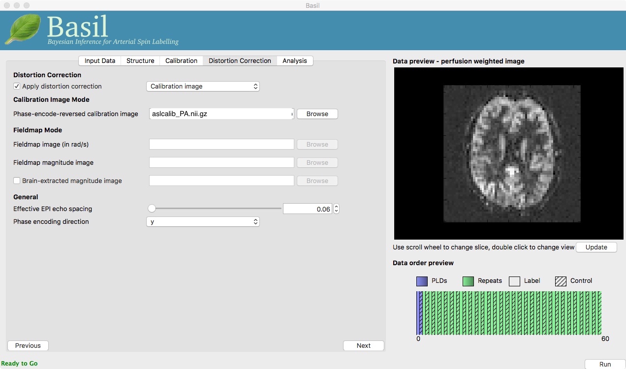
On the ‘Distortion Correction’ tab, select ‘Apply distortion
correction’. Load the ‘Phase-encode-reveresed calibration image’
aslcalib_PA.nii.gz. Set the ‘Effective EPI echo
spacing’ (also known as the dwell time) to 0.95ms and the ‘Phase encoding direction’ to ‘y’.
On the ‘Analysis’ tab, select ‘Motion Correction’. Make sure you have ‘Adaptive spatial regularisation on perfusion’ selected (it is by default). This will reduce the appearance of noise in the final perfusion image using the minimum amount of smoothing appropriate for the data.
You might like the change the name of the output directory at this point, so that you can comapre to the previous analysis.
Now click ‘Run’.

For this analysis we are still in ‘White Paper’ mode. Specifically this means we are using the simplest kinetic model, which assumes that all delivered blood-water has the same T1 as that of the blood and that the Arterial Transit Time should be treated as 0 seconds.
As before, the analysis should only take a few minutes, slightly longer this time due to the distortion and motion correction. Like the last exercise you might want to skip ahead and start setting up the next analysis.
To view the final result:
fsleyes oxasl/output/native/calib_voxelwise/perfusion.nii.gz
The result will be similar to the analysis in Example 1 although the effect of distortion correction should be noticeable in the anterior portion of the brain. The effects of motion correction are less obvious, this data does not have a lot of motion corruption in it.
Making use of Structural Images
Thus far, all of the analyses have relied purely on the ASL data alone. However, often you will have a (higher resolution) structural image in the same subject and would like to use this as well, at the very least as part of the process to transform the perfusion images into some template space.
We can repeat the analysis above but now providing structural
information. The recommended way to do
this is to take your T1 weighted structural image (which is most
common) and firstly process using fsl_anat, passing the
output directly from that tool BASIL.
For this practical fsl_anat has already been run for
you and you will find the output in the data directory as ~/fsl_course_data/ASL/T1.anat
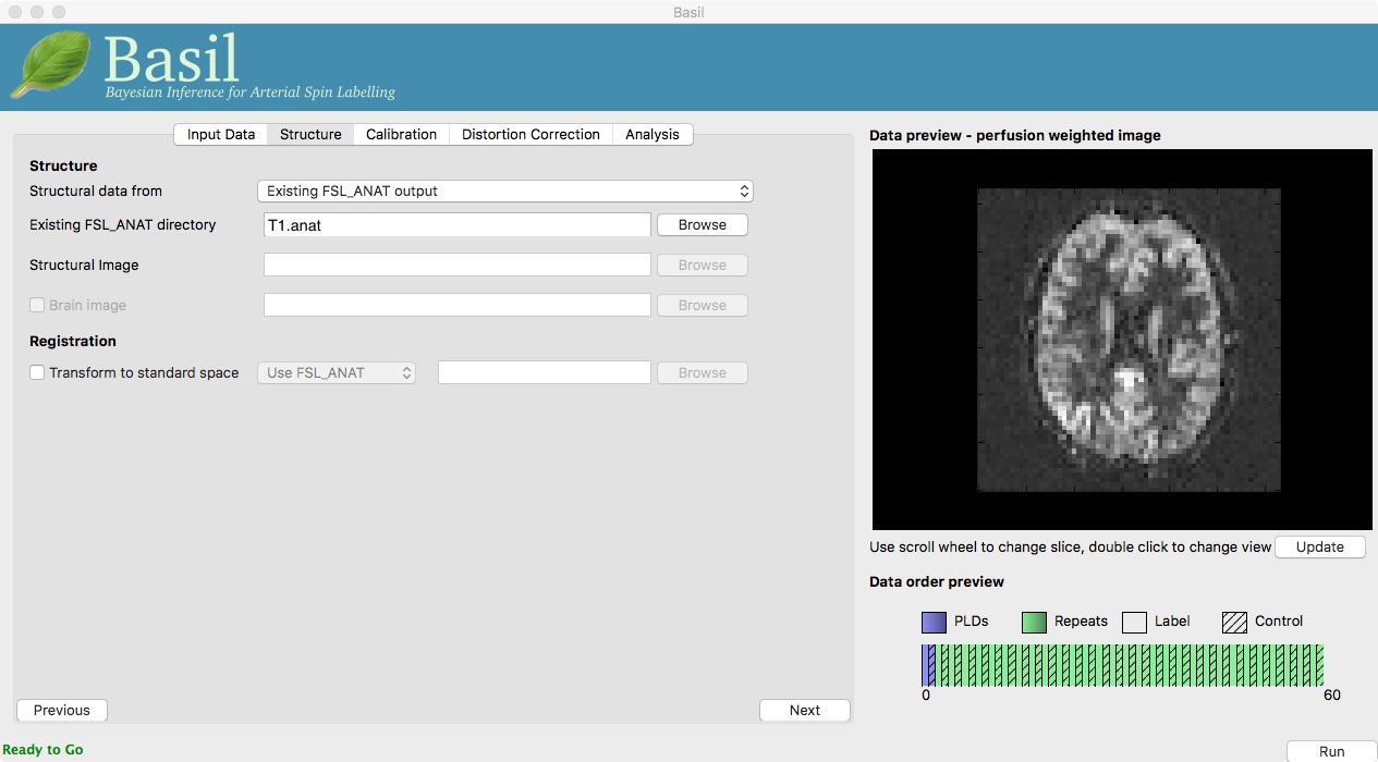
Go back to the analysis you have setup above. On the ‘Structure’
tab, for ‘Structural data from’ select ‘Existing FSL_ANAT
output’. Then for the ‘Existing FSL_ANAT output’ choose
T1.anat.
This analysis will take somewhat longer overall (potentailly 15-20 mins), the extra time is taken up doing careful registration between ASL and structural images. Thus, this is a good point to keep reading on and leave the analysis runnning.
You will find some new results in the output directory:
oxasl/struct_space- this sub-drectory contains results transformed into the same space as the structural image. The files in here will match those in thenativesubdirectory of the earlier analysis, i.e., containing perfusion images with and without calibration.
oxasl/output/native/asl2struct.mat- this is the (linear) transformation between ASL and structural space. It can be used along with a transformation between structural and template space to transform the ASL data into the template space. It was used to create the results inoxasl/output/struct.
oxasl/output/native/perfusion_calib_gm_mean.txt- this contains the result of calculating the perfusion within a gray matter mask, these are in ml/100g/min. The mask was derived from the partial volume estimates created byfsl_anatand transformed into ASL space followed by thresholding at 70%. This is a helpful check on the absolute perfusion values found and it is not aytpical too see values in the range 30-50 here. There is also a white matter result (for which a threshold of 90% was used).
oxasl/output/native/gm_mask.nii.gz- this is the gray matter mask used in the above calculations. There is also the associated white matter mask.
oxasl/output/native/gm_roi.nii.gz- this is another mask that represents areas in which there is some grey matter (at least 10% from the partial volume estimates). This can be useful for visualisation, but mainly when looking at partial volume corrected data.
Different model and calibration choices
Thus far the calibration to get perfsion in units of ml/100g/min has been done using a voxelwise division of the realtive perfusion image by the (suitably corrected) calibration image - so called ‘voxelwise’ calibration. This is in keeping with the recommendations of the ASL White Paper for a simple to implement quantitative analysis. However, we could also choose to use a reference tissue to derive a single value for the equilibrium magnetization of arterial blood and use that in the calibration process.
Go back to the analysis you have already set up. We are now going to turn off ‘White Paper’ mode, this will provide us with more options to get a potentially more accurate analysis. To do this return to the ‘Analysis’ tab and deselect the ‘White Paper’ option, you will see that the ‘Arterial Transit Time’ goes from 0 seconds to 1.3 seconds (the default value for pcASL in BASIL based on our experience with pcASL labeling plane placement) and the ‘T1’ value (for tissue) is different to ‘T1b’ (for arterial blood), since the Standard (aka Buxton) model for ASL kinetics considers labeled blood both in the vascualture and the tissue.
Now that we are not in ‘White Paper’ mode we can also change the calibration method. On the ‘Calibration’ tab, change the ‘Calibration mode’ to ‘Reference Region’. Now all of the ‘Reference tissue’ options will become available, but leave these as they are: we will accept the default option of using the CSF (in the ventricles) for calibration.
You could click ‘Run’ now and wait for the analysis to complete. But, in the interests of time we will save ourselves the bother of doing all of the registration all over again. Before clicking run, therefore, do:
On the ‘Calibration’ tab select ‘Mask’ and load
csfmask.nii.gzfrom the data directory. This is a ready prepared ventricular mask for this subject. (in fact it is precisely the mask you would get if you ran the analysis as setup above).Go back to the ‘Structure’ tab and choose ‘None’ for ‘Structural data from’. This will turn off all of the registration processes.
You might also like to choose a different output directory name, so that you can comapre with the previous analysis.
While this is running you might want to read ahead, or if you are keen to keep moving through the examples, then skip this analysis and keep going.
The resulting perfusion images should look very similar to those
produced using the voxelwise calibration, and the absolute values
should be similar too. For this, and many datasets, the two methods
are broadly equivalent. You can check on some of the interim
calcuations for the calibration by looking in the
oxasl/calib subdirectory: here you will find the value
of the estimated equilirbirum mangetization of arterial blood for
this dataset in M0.txt and the reference tissue mask in
refmask.nii.gz. It is worth checking that the latter
does indeed only lie in the venticles when overlaid on an ASL image
(e.g. the perfusion image or the calibration image), it should be
conservative, i.e., only select voxels well within the ventricles
and not on the boundary with white matter.
Partial Volume Correction
Having dealt with structural image, and in the process obtained partial volume estimates, we are now in a position to do partial volume correction. This does more than simply attempt to estimate the mean perfusion within the grey matter, but attempts to derive and image of gray matter perfusion directly (along with a separate image for white matter).
This is very simple to do via the GUI. Return to your earlier
analysis. You will need
to revist the ‘Structure’ tab and reload the T1.anat
result as you did above, the partial volume estimates produced by
fsl_anant (in fact they are done using fast)
are needed for the correction. On the ‘Analysis’ tab,
select ‘Partial Volume Correction’. That is it! You might not want to
click ‘Run’ at this point becuase partial volume correction takes
substantially longer to run.
You will find the results of this analysis already completed for
you in the directory ~/fsl_course_data/ASL/oxasl_spld_pvout. In this results directory you will still find an analysis performed
without partial volume correction in oxasl/output/native
as before. The results of partial volume correction can be found in
oxasl/output/native/pvcorr. This new subdirectory has the
same structure as the non-corrected results, only now
perfusion_calib.nii.gz is an estimate of perfusion only
in gray matter, it has been joined by a new set of images for the
estimation of white matter perfusion, e.g.,
perfusion_wm_calib.nii.gz. It may be more helpful to look at
perfusion_calib_masked.nii.gz (and the equivalent
perfusion_wm_calib_masked.nii.gz) since this has been
masked to include only voxels with more than 10% gray matter (or white
matter), i.e., voxels in which it is reasonable to interpret the gray
matter (white matter) perfusion values.
Perfusion Quantification (and more) using Multi-PLD pcASL
The purpose of this exercise is to look at some multi-PLD pcASL. As with the single PLD data we can obtain perfusion images, but now we can account for any differences in the arrival of labeled blood-water (the arterial transit time, ATT) in different parts of the brain. As we will also see we can extract other interesting parameters, such as the ATT in its own right, as well as arterial blood volumes.
The data
The data we will use in this section supplements the single PLD pcASL data above, adding multi-PLD ASL in the same subject (collected in the same session). This dataset used the same pcASL labelling, but with a label duration of 1.4 seconds and 6 post-labelling delays of 0.25, 0.5, 0.75, 1.0, 1.25 and 1.5 seconds.
The files you will also now need are:
mpld_asltc.nii.gz- the label-control ASL series containing 96 volumes: each PLD was repeated 8 times, thus there are 16 volumes (label and control paired) for each PLD. The data has been re-ordered from the way it was acquired, such that all of the measurements from each PLD have been grouped together - it is important to know this data ordering when doing the analysis.
Perfusion Quantification
Load the GUI (asl_gui), it is best to start a
whole new analysis as we are moving on to a new set of data and not
reuse any GUI you already have open. On the
‘Input Data’ tab, for the ‘Input Image’ load
mpld_asltc.nii.gz. Unlike the single-PLD data, we need to specify the correct number
of PLD, which is 6. At this point the ‘Number of repeats’ should
correctly read 8. Click ‘Update’ below the ‘Data preview pane’. A
perfusion-weighted image should appear - this is an average over all
the PLDs (and will thus look different to Example 1).
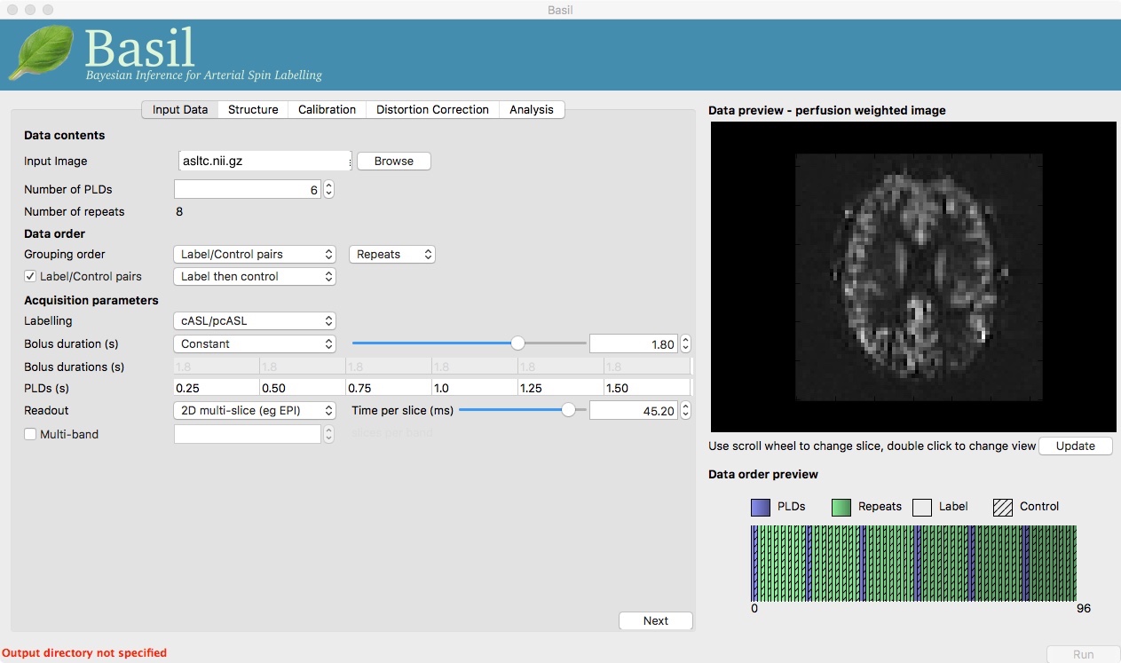
Note the ‘Data order preview’. For mutli-PLD ASL it is important to get the data order specification right. In this case the default options in the GUI are not correct. The PLDs do come as label-control pairs, i.e. alternating label then control images. But, the default assumption in the GUI is that a full set of the 6 PLDs has been acquired first, then this has been repeated 8 subseqeunt times, this is indcated in the preview by colouring the first instance of a PLD as purple and subsequent as green, with different PLDs appearing as different shades of purple (or green). This is quite commonly how multi-PLD ASL data is acquired, but that might not be how the data is ordered in the final image file.
As we noted earlier, in this data all of the measurements at the same PLD are grouped together. You need to change the ‘Grouping order’ on the ‘Input Data’ tab: leave the first option along (‘Label/Control pairs’) and change the second option from ‘PLDs’ to ‘Repeats’. Note that the data order preview changes to reflect the different ordering. This is now correct: remeber that the purple coloured entries indicate the first time that PLD was acquired.
Note that if you were to click ‘Update’ on the ‘Data preview’ nothing
changes, the ordering doesn’t affect the (simple) way in which we
have calucated the PWI. Getting a plausible looking PWI is a good sign that the data
order is correct, but it is not a guarantee that the PLD ordering is
correct, so always check carefully. One way to do this, in this
case, would be to open the data in fsleyes and look at
the timeseries: the raw intensity of both label and control images
for one PLD are different to those from another PLD (due to the
background suprresion). THe timeseries for the raw data looks like a
series of steps, indicating the repeated measurements from each PLD
are grouped together (groubed by ‘repeats’).
Once we are happy with the PWI and data order, we can set the ‘Acquisition parameters’:
Labelling - ‘cASL/pcASL’ (default).
Bolus duration (s) - 1.4 (shorter than the default).
PLDs (s) - 0.25, 0.5, 0.75, 1.0, 1.254, 1.5.
Readout - ‘2D multi-slice’ with ‘Time per slice’ 45.2.
Move to the ‘Calibration’ tab, select ‘Enable Calibration’ and as
the ‘Calibration Image’ load the aslcalib.nii.gz image
from the Single-PLD data (it is from the same subject in the same
session so we can use it here too). We have skipped the ‘Structure’
tab (to make the analysis quicker), this means if we want ‘Calibration
mode’ to be ‘Reference Region’ we need to supply a mask of the
region of tissue to use. Select ‘Mask’ and load
csfmask.nii.gz. Set the ‘Sequence TR’ to be 4.8, but
leave all of the other options alone.
Move to the ‘Distortion Correction’ tab. Select ‘Apply distortion
correction’. Load the ‘Phase-encode-reveresed calibration image’
aslcalib_PA.nii.gz from the Single-PLD pcASL data. Set the ‘Effective EPI echo
spacing’ to 0.95ms again and the ‘Phase encoding direction’ to ‘y’.
Finally, move to the ‘Analysis’ tab. Choose an output directory, leave all of the other options alone. Click ‘Run’.
This analysis shouldn’t take a lot longer than the equivalent single PLD analysis, but feel free to skip ahead to the next section whilst you are waiting.
The results directory from this analysis should look similar to
that obtained for the single PLD pcASL. That is reassuring as it is the same subject. The main difference is the
arrival.nii.gz image. If you examine this image you should find a pattern of values
that tells you the time it takes for blood to transit between the
labeling and imaging regions. You might notice that the
arrival.nii.gz image was present even in the single-PLD
results, but if you looked at it contained a single value - the one
set in the Analysis tab - which meant that it
appeared blank in that case.
Arterial/Macrovascular Signal Correction
In the analysis above we didn’t attempt to model the presence of arterial (macrovascular) signal. This is fairly reasonable for pcASL in general, since we can only start sampling some time after the first arrival of labeled blood-water in the imaging region. However, given we are using shorter PLD in our multi-PLD sampling to improve the SNR there is a much greater likelihood of arterial signal being present. Thus, we might like to repeat the analysis with this component included in the model.
Return to your analysis from before. On the ‘Analysis’ tab select ‘Include macro vascular component’. Click ‘Run’.
The results directory should be almost identical to the previous run, but now we also gain some new results:
aCBV.nii.gzand
aCBV_calib.nii.gz
Following the convention for the perfusion images, these are the relative and absolute arterial (cerebral) blood volumes respectively. If you examine one of these and focus on the more inferior slices you should see a pattern of higher values that map out the structure of the major arterial vasculature, including the Circle of Willis. This finding of an arterial contribution in some voxels results in a correction to the perfusion image - you may now be able to spot that in the same slices where there was some evidence for arterial contamination of the perfusion image before that has now been removed.
Partial Volume Correction
In the same way that we could do partial volume correction for single PLD pcASL, we can do this for multi-PLD. If anything partial volume correction should be even better for multi-PLD ASL, as there is more information in the data to separate grey and white matter perfusion.
Just like the single PLD case we will require structural
information, entered on the ‘Structure’ tab. We can do as we did
before and load T1.anat. On the ‘Analysis’ tab, select
‘Partial Volume Correction’.
Again, this analysis will not be very quick and so you might not wish to click ‘Run’ right now.
You will find the results of this analysis already completed for
you in the directory
~/fsl_course_data/ASL/oxasl_mpld_pvout. This results directory contains, as a further subdirectory, pvcorr,
within the native subdirectory, the partial volume
corrected results: gray matter (perfusion_calib.nii.gz
etc) and white matter perfusion
(perfusion_wm_calib.nii.gz etc)
maps. Alongside these there are also gray and white matter ATT maps
(arrival and arrival_wm respectively). The
estimated maps for the arterial component
(aCBV_calib.nii.gz etc) are still present in the
pvcorr directory. Since this is not tissue specific there
are not separate gray and white matter versions of this parameter.
The End.